
In today’s world, the pursuit of efficiency is essential for businesses, organizations, and individuals alike. Whether it’s about saving time, money, or resources, improving efficiency is often at the core of decision-making processes. But how do we select the most effective measures from a plethora of available options? Enter multi-objective optimization and the knapsack approach – two powerful tools that can help us make informed choices in a sea of alternatives and for Sustainability Optimization.
Multi-objective optimization is an advanced mathematical technique that helps in determining the best possible solutions for complex problems, where multiple conflicting objectives must be considered. Instead of focusing on a single objective, such as minimizing cost or maximizing revenue, multi-objective optimization takes into account several objectives simultaneously. This approach enables decision-makers to find a set of optimal trade-offs that best satisfy their goals, taking into account the various constraints and priorities they may have.
In this blog post, we will explore how multi-objective optimization, combined with the knapsack approach, can be employed to effectively select the most suitable efficiency measures from a wide array of options. By understanding and leveraging these powerful tools, you will be better equipped to make informed, data-driven decisions that lead to improved efficiency and overall success. So, let’s dive in and unlock the potential of multi-objective optimization and the knapsack approach for your efficiency measures selection journey!
Understanding Multi-Objective Optimization
Multi-objective optimization is a powerful mathematical technique that focuses on solving problems with multiple conflicting objectives. In contrast to single-objective optimization, which seeks to optimize a single objective (such as minimizing cost or maximizing profit), multi-objective optimization considers several objectives simultaneously. By doing so, it provides decision-makers with a set of optimal trade-offs that best satisfy their goals, given the constraints and priorities they have.
Pareto optimality and the Pareto front
Central to the concept of multi-objective optimization is the notion of Pareto optimality. A solution is considered Pareto optimal if there is no other solution that can improve one objective without worsening at least one other objective. In other words, a Pareto optimal solution represents the best possible trade-off among the conflicting objectives.
The set of all Pareto optimal solutions forms what is known as the Pareto front. The Pareto front is a valuable tool for decision-makers, as it provides a visual representation of the trade-offs between the different objectives. By analyzing the Pareto front, decision-makers can gain insights into the relationships between the objectives and make informed choices that best align with their goals and preferences.
Benefits and applications of multi-objective optimization
There are several benefits to using multi-objective optimization in decision-making processes. Some of these benefits include:
- Comprehensive solutions: By considering multiple objectives simultaneously, multi-objective optimization provides a more comprehensive understanding of the problem at hand, helping decision-makers identify the most suitable solutions.
- Flexibility: Multi-objective optimization allows decision-makers to explore various trade-offs and adapt to changing priorities, making it a flexible and versatile approach.
- Informed decision-making: The Pareto front provides a clear visualization of the relationships between the objectives, enabling decision-makers to make more informed choices based on their preferences and goals.
Multi-objective optimization is used in a wide range of applications, including engineering design, finance, environmental management, and healthcare, among others. Its versatility and effectiveness make it a valuable tool for addressing complex, real-world problems.
The Knapsack Approach
The knapsack approach, often referred to as the knapsack problem, is a classic combinatorial optimization problem that arises in various resource allocation scenarios. The problem can be simply described as follows: Given a set of items, each with a weight and a value, determine the combination of items that can be placed in a knapsack (with a limited capacity) to maximize the total value without exceeding the knapsack’s weight capacity.
One of the most well-known versions of the knapsack problem is the 0/1 knapsack problem. In this variant, each item can either be included in the knapsack or not (represented by 0 or 1), with no possibility of splitting or fractional inclusion. The 0/1 knapsack problem can be formally defined as follows:
Given:
- A set of n items, each with a weight w_i and a value v_i (i = 1, 2, …, n)
- A knapsack with a maximum weight capacity W
Objective:
- Maximize the total value of the selected items, subject to the constraint that the total weight of the selected items does not exceed W.
Solving the knapsack problem using dynamic programming and greedy algorithms
There are various algorithms and techniques for solving the knapsack problem, including dynamic programming, greedy algorithms, and more advanced approaches such as branch and bound or genetic algorithms.
Dynamic programming is a powerful technique for solving the 0/1 knapsack problem, particularly when the problem size is not too large. This approach involves building a table that represents the optimal solutions for smaller subproblems, using these solutions to construct the optimal solution for the original problem. The dynamic programming algorithm typically has a time complexity of O(nW), where n is the number of items and W is the knapsack capacity.
Greedy algorithms, on the other hand, offer a simpler, more intuitive approach to solving the knapsack problem. These algorithms involve iteratively selecting items based on a specific criterion, such as the value-to-weight ratio, until the knapsack’s capacity is reached or no more items can be added. While greedy algorithms are generally faster than dynamic programming, they do not guarantee finding the optimal solution in all cases, especially when the problem is more complex.
Combining Multi-Objective Optimization and the Knapsack Approach
The multi-objective knapsack problem (MOKP)
When it comes to selecting efficiency measures, or Sustainability Optimization, the combination of multi-objective optimization and the knapsack approach can be incredibly powerful. This hybrid approach leads to the multi-objective knapsack problem (MOKP), which extends the classic knapsack problem to consider multiple conflicting objectives. In MOKP, each item is associated with multiple values, representing different objectives that need to be optimized simultaneously.
How MOKP helps in selecting efficiency measures
The multi-objective knapsack problem is particularly well-suited for selecting efficiency measures, as it allows decision-makers to consider various factors and trade-offs when choosing the best combination of measures. By incorporating multiple objectives, such as cost savings, environmental impact, and resource usage, MOKP enables decision-makers to identify the most suitable efficiency measures that align with their goals and constraints.
Solving the multi-objective knapsack problem can be more challenging than its single-objective counterpart due to the added complexity of multiple objectives. However, various algorithms have been developed specifically for tackling multi-objective optimization problems, including MOKP. Some popular algorithms for solving MOKP are:
- Genetic Algorithms: These are nature-inspired optimization algorithms based on the principles of natural selection and genetics. They involve creating a population of potential solutions, which then evolve through processes like selection, crossover, and mutation to find the optimal solution. Genetic algorithms have proven to be effective in solving MOKP, particularly for large-scale and complex problems.
- NSGA-II (Non-dominated Sorting Genetic Algorithm II): NSGA-II is a popular multi-objective optimization algorithm that extends the concept of genetic algorithms. It uses a non-dominated sorting approach to rank potential solutions based on their Pareto optimality, and a crowding distance metric to maintain diversity within the population. NSGA-II is highly effective in solving MOKP and has been widely applied in various domains.
By utilizing these algorithms, decision-makers can efficiently find the best combinations of efficiency measures that meet their multiple objectives and constraints.
Real-World Examples and Applications
One prominent application of the multi-objective knapsack problem in selecting efficiency measures is in the field of energy efficiency for buildings. Building owners and facility managers often face the challenge of selecting the most effective combination of energy efficiency measures (EEMs) to minimize energy consumption, reduce greenhouse gas emissions, and decrease operating costs while adhering to budget constraints.
The multi-objective knapsack problem can help decision-makers address this challenge by considering multiple objectives, such as energy savings, cost-effectiveness, and environmental impact, when selecting EEMs. By using algorithms like genetic algorithms or NSGA-II, they can identify the optimal combination of EEMs that best align with their goals and constraints.
Examples of EEMs in this context include upgrading insulation, installing energy-efficient lighting systems, optimizing HVAC systems, and implementing building automation systems. By applying the MOKP approach to analyze and compare the trade-offs between these measures, building owners and facility managers can make more informed decisions to improve energy efficiency and reduce their overall environmental footprint.
Energy efficiency measures for buildings: A hypothetical case study
Let’s consider a hypothetical situation in which a business plans to construct a new 10,000 square foot office building. They are committed to sustainability and have allocated $250,000 towards implementing energy efficiency measures (EEMs).
For the purpose of this example, we will make the following realistic assumptions regarding the first cost, annual energy cost savings, and annual CO2 reduction for each option:
(Note: The values provided below are for illustration purposes only and may vary based on various factors such as location, building design, local energy prices, and more.)
- High-efficiency lighting
- First cost: $30,000
- Annual energy cost savings: $5,000
- Annual CO2 reduction: 10 tons
- Solar panels
- First cost: $80,000
- Annual energy cost savings: $8,000
- Annual CO2 reduction: 15 tons
- Increased thermal insulation
- First cost: $40,000
- Annual energy cost savings: $4,000
- Annual CO2 reduction: 8 tons
- High U-value windows
- First cost: $60,000
- Annual energy cost savings: $3,000
- Annual CO2 reduction: 6 tons
- Water-source heat pumps with geothermal fields
- First cost: $100,000
- Annual energy cost savings: $12,000
- Annual CO2 reduction: 25 tons
- Air source heat pumps
- First cost: $50,000
- Annual energy cost savings: $6,000
- Annual CO2 reduction: 12 tons
- Wind turbines
- First cost: $120,000
- Annual energy cost savings: $10,000
- Annual CO2 reduction: 20 tons
- LED lighting control system
- First cost: $20,000
- Annual energy cost savings: $3,000
- Annual CO2 reduction: 5 tons
- Cool roofs (reflective roofing materials)
- First cost: $50,000
- Annual energy cost savings: $2,500
- Annual CO2 reduction: 7 tons
- Energy-efficient HVAC system (Variable Refrigerant Flow)
- First cost: $120,000
- Annual energy cost savings: $10,000
- Annual CO2 reduction: 20 tons
- Energy recovery ventilation system
- First cost: $40,000
- Annual energy cost savings: $4,000
- Annual CO2 reduction: 8 tons
- Building automation system (BAS)
- First cost: $60,000
- Annual energy cost savings: $6,000
- Annual CO2 reduction: 12 tons
- Rainwater harvesting system
- First cost: $30,000
- Annual energy cost savings (for water pumping): $1,000
- Annual CO2 reduction: 2 tons
- Green walls and roof gardens
- First cost: $70,000
- Annual energy cost savings (for heating and cooling): $2,000
- Annual CO2 reduction: 4 tons
Using MOKP, the business can maximize energy savings and emission reduction while staying within their $250,000 budget. By defining the multiple objectives (energy savings and CO2 reduction) and constraints (budget), the MOKP can be used to find the optimal combination of EEMs that provides the best balance between energy savings, emissions reduction, and cost.
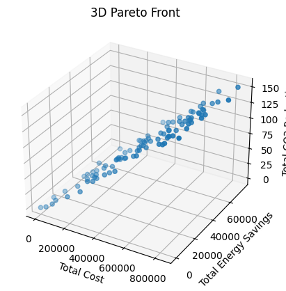
In this case, the decision-makers can apply an algorithm like NSGA-II to generate a Pareto front that represents the various trade-offs between energy savings, CO2 reduction, and cost. By analyzing the Pareto front, the business can identify the combination of EEMs that best aligns with their sustainability goals and budget constraints.
For example, they might find that a combination of high-efficiency lighting, solar panels, and increased thermal insulation provides the best balance of energy savings, CO2 reduction, and cost within their budget. By using MOKP, the business can make a more informed decision when selecting EEMs, ultimately contributing to a sustainability optimized and energy-efficient building. Now that we have identified the problem and proposed an approach, MOKP, we will demonstrate the Python code to solve the multi-objective knapsack problem. We will utilize the DEAP (Distributed Evolutionary Algorithms in Python) library, which is a powerful and flexible library for designing and solving evolutionary algorithms. More information about DEAP can be found at the Github Repository: https://github.com/DEAP/deap
We will walk you through the following steps:
- Installing the DEAP library
- Defining the problem, including the energy efficiency measures, budget constraint, and objectives
- Creating the necessary types and functions for the problem, such as the evaluation function and random individual generator
- Setting up the DEAP toolbox to configure the selection, crossover, and mutation operators
- Running the optimization and analyzing the Pareto front to find the optimal combination of energy efficiency measures
Python Code
!pip install deap
import random
import numpy as np
from deap import base, creator, tools, algorithms
# Define the problem
EEMs = [
{“name”: “High-efficiency lighting”, “cost”: 30000, “savings”: 5000, “co2_reduction”: 10},
{“name”: “Solar panels”, “cost”: 80000, “savings”: 8000, “co2_reduction”: 15},
{“name”: “Increased thermal insulation”, “cost”: 40000, “savings”: 4000, “co2_reduction”: 8},
{“name”: “High U-value windows”, “cost”: 60000, “savings”: 3000, “co2_reduction”: 6},
{“name”: “Water-source heat pumps with geothermal fields”, “cost”: 100000, “savings”: 12000, “co2_reduction”: 25},
{“name”: “Air source heat pumps”, “cost”: 50000, “savings”: 6000, “co2_reduction”: 12},
{“name”: “Wind turbines”, “cost”: 120000, “savings”: 10000, “co2_reduction”: 20},
{“name”: “LED lighting control system”, “cost”: 20000, “savings”: 3000, “co2_reduction”: 5},
{“name”: “Cool roofs”, “cost”: 50000, “savings”: 2500, “co2_reduction”: 7},
{“name”: “Energy-efficient HVAC system (VRF)”, “cost”: 120000, “savings”: 10000, “co2_reduction”: 20},
{“name”: “Energy recovery ventilation system”, “cost”: 40000, “savings”: 4000, “co2_reduction”: 8},
{“name”: “Building automation system (BAS)”, “cost”: 60000, “savings”: 6000, “co2_reduction”: 12},
{“name”: “Rainwater harvesting system”, “cost”: 30000, “savings”: 1000, “co2_reduction”: 2},
{“name”: “Green walls and roof gardens”, “cost”: 70000, “savings”: 2000, “co2_reduction”: 4},
]
BUDGET = 500000
# Create types
creator.create(“FitnessMulti”, base.Fitness, weights=(1.0, 1.0))
creator.create(“Individual”, list, fitness=creator.FitnessMulti)
# Initialize functions
def random_individual():
return [random.randint(0, 1) for _ in range(len(EEMs))]
def evaluate(individual):
cost = sum(EEMs[i][“cost”] for i in range(len(EEMs)) if individual[i])
if cost > BUDGET:
return -1e9, -1e9 # Penalize if budget constraint is violated
savings = sum(EEMs[i][“savings”] for i in range(len(EEMs)) if individual[i])
co2_reduction = sum(EEMs[i][“co2_reduction”] for i in range(len(EEMs)) if individual[i])
return savings, co2_reduction
toolbox = base.Toolbox()
toolbox.register(“individual”, tools.initIterate, creator.Individual, random_individual)
toolbox.register(“population”, tools.initRepeat, list, toolbox.individual)
toolbox.register(“mate”, tools.cxTwoPoint)
toolbox.register(“mutate”, tools.mutFlipBit, indpb=0.1)
toolbox.register(“select”, tools.selNSGA2)
toolbox.register(“evaluate”, evaluate)
# Run the optimization
random.seed(42)
population = toolbox.population(n=100)
result, logbook = algorithms.eaSimple(population, toolbox, cxpb=0.8, mutpb=0.2, ngen=100, verbose=False)
# Get the Pareto front
pareto_front = tools.sortLogNondominated(result, len(result))
# Print the results
print(“Pareto front:”)
for individual in pareto_front[0]:
print(“Selected EEMs: “, [EEMs[i][“name”] for i in range(len(EEMs)) if individual[i]])
print(“Total cost: “, sum(EEMs[i][“cost”] for i in range(len(EEMs)) if individual[i]))
print(“Total energy savings: “, sum(EEMs[i][“savings”] for i in range(len(EEMs)) if
individual[i]))
print(“Total CO2 reduction: “, sum(EEMs[i][“co2_reduction”] for i in range(len(EEMs)) if individual[i]))
print()
# Find and print the best solution (if multiple solutions have the same fitness, choose the first one)
best_solution = pareto_front[0][0]
best_fitness = best_solution.fitness.values
for individual in pareto_front[0]:
if individual.fitness.values == best_fitness:
best_solution = individual
break
print(“Best solution:”)
print(“Selected EEMs: “, [EEMs[i][“name”] for i in range(len(EEMs)) if best_solution[i]])
print(“Total cost: “, sum(EEMs[i][“cost”] for i in range(len(EEMs)) if best_solution[i]))
print(“Total energy savings: “, sum(EEMs[i][“savings”] for i in range(len(EEMs)) if best_solution[i]))
print(“Total CO2 reduction: “, sum(EEMs[i][“co2_reduction”] for i in range(len(EEMs)) if best_solution[i]))
# Extract the objective values for all individuals in all Pareto fronts
costs = []
savings = []
co2_reductions = []
for front in pareto_front:
for individual in front:
costs.append(sum(EEMs[i][“cost”] for i in range(len(EEMs)) if individual[i]))
savings.append(sum(EEMs[i][“savings”] for i in range(len(EEMs)) if individual[i]))
co2_reductions.append(sum(EEMs[i][“co2_reduction”] for i in range(len(EEMs)) if individual[i]))
# Create a 3D scatter plot
fig = plt.figure()
ax = fig.add_subplot(111, projection=’3d’)
ax.scatter(costs, savings, co2_reductions)
ax.set_xlabel(‘Total Cost’)
ax.set_ylabel(‘Total Energy Savings’)
ax.set_zlabel(‘Total CO2 Reduction’)
plt.title(‘3D Pareto Front’)
plt.show()
Knapsack Optimization Results
The DEAP algorithm has found an optimal solution that includes the following energy efficiency measures (EEMs) for the 10,000 square foot building, given the specified budget constraint:
- High-efficiency lighting: This measure reduces energy consumption by using energy-efficient light sources, resulting in both energy and cost savings.
- Air source heat pumps: These heat pumps transfer heat between the building and the outdoor air, providing efficient heating and cooling and reducing energy consumption and CO2 emissions.
- Cool roofs: By reflecting more sunlight and absorbing less heat, cool roofs decrease the building’s cooling needs, resulting in energy savings and a reduced carbon footprint.
- Energy recovery ventilation system: This system exchanges energy between incoming and outgoing airstreams, improving indoor air quality and reducing the energy required for heating and cooling.
- Building automation system (BAS): A BAS integrates and controls various building systems, such as HVAC, lighting, and security, optimizing energy consumption and improving overall efficiency.
The DEAP algorithm selected these five options out of the available energy efficiency measures as they collectively provide the greatest energy savings while staying within the budget. By implementing these measures, the building will achieve a significant reduction in energy consumption and CO2 emissions, leading to improved sustainability and environmental performance.
Out of the 14 energy efficiency measures considered, the DEAP algorithm selected these five options as they collectively provide the greatest energy savings while staying within the budget. The total energy savings achieved by implementing these measures is 23,500, and the CO2 saved amounts to 49 tons. This combination of EEMs ensures a significant reduction in energy consumption and a substantial decrease in CO2 emissions, leading to a more sustainable building and improved environmental performance.
In conclusion, the use of multi-objective optimization and the knapsack approach is a powerful tool for making informed decisions when selecting energy efficiency measures for your sustainable building projects. By utilizing this “Sustainability Optimization” technique, you can balance cost, energy savings, and CO2 reduction objectives to find the most effective combination of measures that suit your specific needs and constraints. This approach allows stakeholders to make better decisions and achieve their sustainability goals without compromising on performance or financial viability. As the world moves towards a greener future, such optimization techniques will become increasingly valuable in helping us design and construct more sustainable buildings for a better tomorrow.
For more in-depth Multi-objective optimization research you can check out prior research here.

Leave a comment